I get a lot of email regarding my use of statistics in predicting market behavior.  The most frequent question by far has to do with a pattern I refer to metaphorically in my book as the Baltimore Chop.  The trading pattern is named for a John McGraw batting trick perfected in the 1890â�,��"�s.  Essentially, this rather noteworthy Baltimore Oriole made a habit of hitting the ball sharply into the ground in front of home plate, so that it would take a bounce above the pitcherâ�,��"�s head and stay uncatchable until the batter was on first base. This spike followed by a pop in the opposite direction reminded me very much of the behavior exhibited by stocks on a strong gap open, and hence the idea for the pattern.

While the idea of fading gaps might be nothing new, my underlying methodology gives the Baltimore Chop a statistical edge that makes me more comfortable about taking a contra trend trade.  By using some basic statistics, I am able to identify gap openings that have a very high probability of reversing and generating profits on the fade.  Iâ�,��"�ll give a specific example of how the setup presents itself a little later.  First, I would like to address the statistic itself, since this seems to be the source of a bit of confusion.

Standard Deviation

Statistical tools, whether simple like means testing (reversion to the mean, multiple regression, etc.) or complicated as in the case of component factors analysis, rely on assumptions.  In the case of short-term stock market data, the most important of these, a normal distribution, is generally met.  What this means in a nutshell is that prices, volatility, range or whatever market behavior you are interested in measuring, tend to have values that plot well within a bell shaped or normally distributed curve.  Most data points will fall around the arithmetic average or mean, thus creating the highest point which is represented in the center of the plot.  As we approach the tails of the distribution, progressively fewer observations will exist, as we are deviating from the central tendency and there is a high probability of these to move back toward the mean. 

The standard deviation (SD) allows us to assess dispersion around the mean and to draw some inferences as to whether a reversion is likely.   Moreover, it allows us to create bands of probabilities that indicate whether a data point might be extended so far from the average that a move in the opposite direction is likely.  The calculation is relatively straight forward and is as follows:

So letâ�,��"�s say that a data point for us is going to be True Range (TR) and that we are interested in Average True Range (ATR) over a period of ten days.  What we are going to do to get one standard deviation is take each of the TR values individually, subtract the ATR value and square the result to get rid of any negative number.  Next, add these values together, divide by ten (the number of days we are looking at), and then take the square root of this number to get rid of the square we introduced a second ago.  Voila, the worst is over, you have just calculated the standard deviation. 

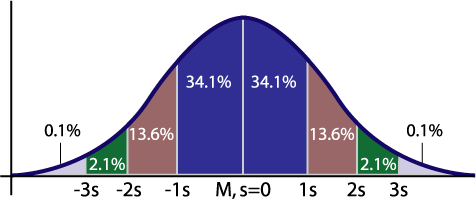
The histogram below shows the percentage of observations we can expect to see one standard deviation above and below the mean ( -1 and +1 SD = 34.1 + 34.1 = 68.2%), two standard deviations above and below the mean ( -2 and +2 SD 68.2 + 13.6 + 13.6 = 95.4%) and three standard deviations above and below the mean ( +3 and -3 SD = 95.4 + 2.1 + 2.1 = 99.6%).  Deriving the second and third SD levels is as easy as multiplying SD by two and three respectively.

OII - A Trading Example

I will use a trade in Oceaneering International (OII) on May 5, 2006 as an example of how the logic follows through. Although I use several measures of volatility to statistically gauge gap reversal probabilities, True Range is my favorite proxy for volatility when performing the calculation because the data are so easy to calculate.  The TR values for the ten days leading up to the gap trade in OII are as follows:

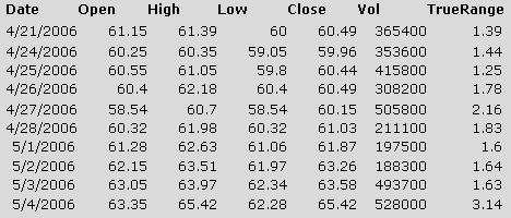
The ATR value is:   

Thus, the standard deviation is:

Adding SD (.54) to the ATR (1.79) and then to the close on May 4, 2006 accounts for 68% of the variability we would expect to see in TR for OII on May 5, 2006.  If we multiply SD by 2 and add it to ATR we get 1.08 + 1.79 = 2.87.  Add this value to the May 4, 2006 close, we will have accounted for 95% of the expected variability in TR. Subtracting these values from the May 4 low establishes the lower bands.

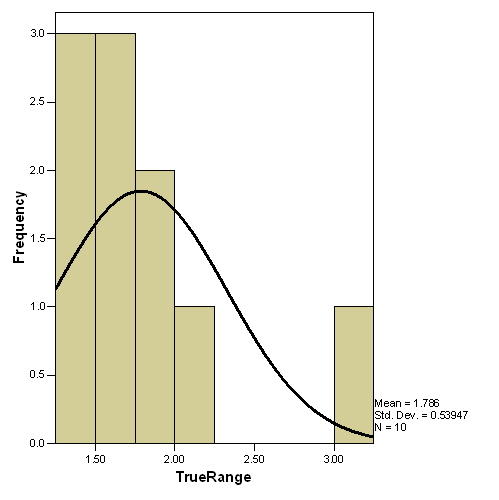
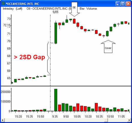
The standard deviation for OII is skewed due to the May 4, 2006 outlier. The rest of the distribution tells us that the distribution is steep, with a strong tendency for TR to gravitate toward the average.  So when our software alerted us that the gap open on May 5, 2006 represented a move of better than 2SD, Julie and I were eager to get short and capitalize on the fact that almost all of the expected opening range had been statistically accounted for. 

I always allow one five minute bar to form prior to taking one of these trades.  My entry is either on a break of the low (high for longs) of the first bar, or on a break of the low (high for longs) of the highest subsequent low.  Essentially, I am either looking for a break of the opening range, or a move that develops after a bit of a pullback.  In the case of OII, we had a pullback entry followed by a move of about $2 per share in just about an hour.  Not bad considering most of the difficult work was done by the math!

As some of you have noted in your emails and private messages, I trade gaps using several different entry criterion.  The Baltimore Chop setup is my favorite because it provides a level of confidence that I donâ�,��"�t get by simply â�,��"eyeballingâ�,� a chart or looking at moving average or pivot support/resistance.  ATR and SD are a nice combination, but they are just one of many statistical volatility filtering techniques that can give you an edge in your trading.

Adrian Manz is the author of Around The Horn: A Trader's Guide To Consistently Scoring In The Markets and is cofounder of TraderInsight.com. Email him at adrian@traderinsight.com.